The following is a popular brain teaser problem about probability.
Randomly select two points on a unit stick to break it into 3 pieces, what is the probability that the 3 pieces can form a triangle?
The critical thing here is how are the two points selected. The most popular (and probably default) way is that , where and are the distances from the two points to the left end of the stick. There some other interesting ways of selecting the points, and I will study the 3 cases in this post.
Independent Uniformly Distributed
Let and be the distances from the two points to the left end of the stick. In this situation we assume that
Method I: Exclusive Method
Let , and be the lengths of the 3 pieces from the left end of the stick. To form a triangle, , and have to satisfy the following conditions.
Or equivalently, $$
\begin{align} P_{\bigtriangleup} &= P(0 < l_1, l_2, l_3 < \frac{1}{2}) \nonumber \newline &= 1 - P(l_1 \ge \frac{1}{2} | l_2 \ge \frac{1}{2} | l_3 \ge \frac{1}{2}) \nonumber \newline &= 1 - \left(P(l_1 \ge \frac{1}{2}) + P(l_2 \ge \frac{1}{2}) + P(l_3 \ge \frac{1}{2})\right). \nonumber \newline \end{align}
\begin{align} P(l_1 \ge \frac{1}{2}) &= P(min\{X_1, X_2\} \ge \frac{1}{2}) = P(X_1 \ge \frac{1}{2}, X_2 \ge \frac{1}{2}) \nonumber \newline &= P(X_1 \ge \frac{1}{2}) P(X_2 \ge \frac{1}{2}) \nonumber \newline &= \frac{1}{2} \times \frac{1}{2} = \frac{1}{4}. \nonumber \end{align}
is symmetric to , so .
It can be shown (see Method II) that , so \begin{align} P_{\bigtriangleup} &= 1 - \left(P(l_1 \ge \frac{1}{2}) + P(l_2 \ge \frac{1}{2}) + P(l_3 \ge \frac{1}{2})\right) \nonumber \newline &= 1 - \left(\frac{1}{4} + \frac{1}{4} + \frac{1}{4}\right) = \frac{1}{4} = 0.25. \nonumber \end{align}
Method II: Visualization
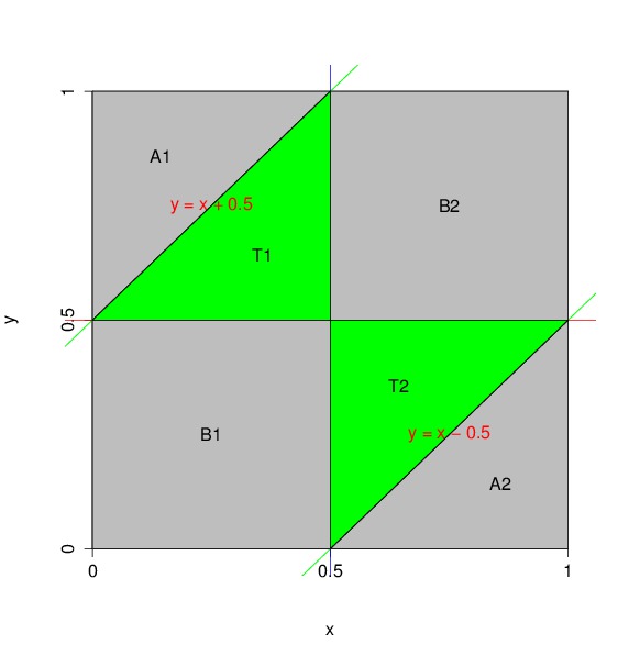
Figure 1: Probability to Form a Triangle.
Let and be defined as above. For the convenience of visualization, Figure 1 uses to stand for and to stand for . The pair is uniformly distributed in the unit square as shown in Figure 1. To form a triangle, and need to satisfy the following conditions. \begin{align} |X - Y| &< \frac{1}{2}, \newline (X - \frac{1}{2}) & (Y - \frac{1}{2}) < 0 \end{align}
Condition (1) requires that the middle part of the 3 pieces cannot be greater than . It is equivalent to \begin{align} Y &> x - \frac{1}{2}, \newline Y &< x + \frac{1}{2}, \end{align} which corresponds to the hexagon in the middle of the unit square (consisting of , , and ). Condition (2) requires that and cannot be both smaller than or bother greater than , which excludes areas and . So when and falls into or (grean areas), the 3 pieces of sticks can form a triangle. It is easy to see that the area/probability is .
Let , and be defined as in Method I. corresponds to the area whose area/probability is ; corresponds to the areas and . Their areas/probabilities sums to . corresponds to the area whose area/probability is .
The R code used to generate Figure 1 is given below.
par(col="black", lty="solid")
# an empty plot without axes
plot(c(0,1), c(0,1), type="n", axes=F, xlab="x", ylab="y")
# add a square
rect(0, 0, 1, 1)
# add x and y axes
at = c(0, 1/2, 1)
lab = c("0", "0.5", "1")
axis(1, pos=0, at=at, labels=lab)
axis(2, pos=0, at=at, labels=lab)
# add 2 green lines with slope 1
abline(1/2, 1, col="green")
abline(-1/2, 1, col="green")
# add a vertical line
abline(v=1/2, col="blue")
# add a horizontal line
abline(h=1/2, col="red")
# top left triangle, grayed
x = c(0, 0, 1/2)
y = c(1, 1/2, 1)
polygon(x, y, col="gray")
# bottom right triangle, grayed
x = c(0.5, 1, 1)
y = c(0, 0, 0.5)
polygon(x, y, col="gray")
# bottom left and top right squares, grayed
x = c(0, 1/2, 1/2, 1, 1, 0)
y = c(0, 0, 1, 1, 1/2, 1/2)
polygon(x, y, col="gray")
# add 2 inner green triangles
x = c(0, 1, 1/2, 1/2)
y = c(1/2, 1/2, 0, 1)
polygon(x, y, col="green")
# flag the top left gray triangle as A1
text(1/7, 6/7, labels="A1")
# flag the bottom right gray triangle as A2
text(6/7, 1/7, labels="A2")
# flag the bottom left gray square as B1
text(1/4, 1/4, labels="B1")
# flag the top right gray square as B2
text(3/4, 3/4, labels="B2")
# flag the 2 inner green triangles as T1 and T2
text(1/2-1/7, 1/2+1/7, labels="T1")
text(1/2+1/7, 1/2-1/7, labels="T2")
# label the (upper) green line y = x + 0.5
text(1/4, 3/4, labels="y = x + 0.5", col="red")
# label the (lower) green line y = x - 0.5
text(3/4, 1/4, labels="y = x - 0.5", col="red")
Method III: Order Statistics
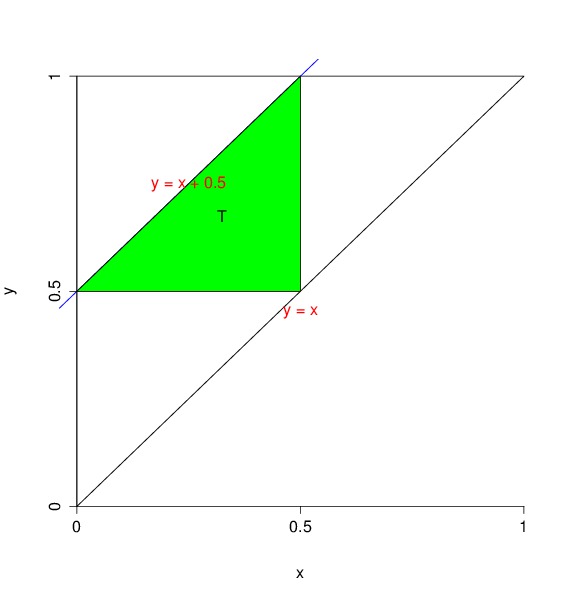
Figure 2: Probability to Form a Triangle.
Let $X_1$ and $X_2$ be as defined above. Let $X_{(1)} = min\{X_1, X_2\}$ and $X_{(2)} = max\{X_1, X_2\}$, then $X_{(1)}$ and $X_{(2)}$ are order statistics. From the theorem of order statistics we know that the join density of $X_{(1)}$ and $X_{(2)}$ is constant 2 with support $0 < X_{(1)} < X_{(2)} < 1$. To form an triangle, $X_{(1)}$ and $X_{(2)}$ have to satisfy the following condition. $$ 0 < x_{(1)} < \frac{1}{2} < X_{(2)} < X_{(1)} + \frac{1}{2}. $$ The probability for the 3 pieces of sticks to form an triangle is thus
\begin{equation}
\int_{0}^{\frac{1}{2}} \int_{\frac{1}{2}}^{x_1+\frac{1}{2}} 2, dx_2,dx_1
= \int_{0}^{\frac{1}{2}} 2x_1 dx_1 = x_1^2|_{0}^{\frac{1}{2}} = \frac{1}{4}.
\end{equation}
The support of the joint density of and is the big triangle in Figure 2. For the convenience of visualization, Figure 2 uses to stand for and to stand for . The integral domain of (5) is the green area T in Figure 2.
The R code to generate Figure 2 is given below.
par(col="black", lty="solid")
plot(c(0,1), c(0,1), type="n", axes=F, xlab="x", ylab="y")
x = c(0, 0, 1)
y = c(1, 0, 1)
polygon(x, y)
segments(1/2, 1, 1/2, 1/2, col="red")
segments(0, 1/2, 1/2, 1/2, col="red")
abline(1/2, 1, col="blue")
at = c(0, 1/2, 1)
lab = c("0", "0.5", "1")
axis(1, pos=0, at=at, labels=lab)
axis(2, pos=0, at=at, labels=lab)
# middle triangle
x = c(0, 1/2, 1/2)
y = c(1/2, 1/2, 1)
polygon(x, y, col="green")
text(1.3/4, 2.7/4, labels="T")
text(1/4, 3/4, labels="y = x + 0.5", col="red")
text(1/2, 0.45, labels="y = x", col="red")
Dependent Uniformly Distributed
Let and be defined as above.
In this situation we assume that
$$
\begin{align}
P_{\bigtriangleup} &= \int_{0}^{\frac{1}{2}} \frac{1}{1-x_1} \int_{\frac{1}{2}}^{x_1+\frac{1}{2}} dx_2, dx_1 \nonumber \newline
&= \int_{0}^{\frac{1}{2}} \frac{x_1}{1-x_1}dx_1 = log2 - \frac{1}{2} \approx 0.1931. \nonumber
\end{align}
The Dirichlet distribution is a distribution that is frequently used in Bayesian non-parametric models. It has a stick-breaking construction. Let , and . The specification of the joint distribution of and sounds a lot like a the construction of a Dirichlet distribution, however, it is not! Given , if , where , then the joint distribution of , and is Dirichlet distribution with concentration parameters 1, and .
Dirichlet Distributed
Let , and be defined as above. In this situation we assume that $$ \begin{align} P_{\bigtriangleup} &= \int_{0}^{\frac{1}{2}} \int_{\frac{1}{2}-x_1}^{\frac{1}{2}} \frac{1}{\pi} x_2^{1/2}(1-x_1-x_2)^{1/2} dx_2, dx_1 \nonumber \newline &= \frac{2}{\pi} - \frac{1}{2} \approx 0.1366. \nonumber \end{align}